Quantum · Qiskit · Real hardware
Quantum Computing on Real IBM Hardware
A Qiskit project that doesn't just simulate — it runs on a real 156-qubit IBM Quantum processor. It executes a Bell state on the QPU and trains a quantum-kernel SVM, then this page lets you play with two genuinely live, in-browser quantum simulators built from scratch in JavaScript.
Overview
Most "quantum" demos online are pure simulation. This one is backed by real silicon: using IBM's free Open Plan, the project submits circuits to an actual superconducting quantum processor and reads back the (noisy) results. Two experiments run end to end — a maximally-entangled Bell state, and a hybrid quantum-classical machine-learning model whose kernel is computed by a quantum circuit. Everything below the fold runs live in your browser on a small statevector simulator I wrote in JavaScript, so you can build circuits and watch quantum mechanics happen with no install.
Live demo · Circuit Lablive
A real 3-qubit statevector simulator. Toggle gates to build a circuit; the bars show the exact measurement probabilities (quantum mechanics, computed live), and you can sample shots — optionally with simulated hardware noise, just like the real QPU.
Build a circuit
Presets:
Or toggle individual gates:
Entangling gates (CNOT):
Measurement
Hardware noise: 0%
Live demo · Quantum-Kernel Classifierlive
This is the heart of the ML experiment, running live. A ZZ-feature-map circuit maps each 2D point to a quantum state; the kernel is the overlap |⟨φ(x)|φ(y)⟩|² between two such states. A kernel-weighted classifier then separates two interleaving "moons". Move your mouse over the plot to classify any point, and drag the encoding scale slider to find the sweet spot — and break it at both ends.
The lesson we actually found
Encoding scale:
There's a sweet spot. Too narrow and every point maps to nearly the same state — the kernel can't tell them apart, so the whole plot guesses one class. Too wide and the states become nearly orthogonal: the kernel matrix collapses toward the identity (kernel concentration) and the boundary dissolves into noise. Both failure modes are real, well-known limitations of quantum machine learning — and you can watch them happen.
Cyan = class A · Magenta = class B · ● = training points · ◇ = your cursor
...and the same code, on a real quantum computer
The browser demos use an exact simulator. The Python project runs the same ideas on IBM's hardware via qiskit-ibm-runtime. Here are the actual results.
Bell state on ibm_fez (156 qubits)
A perfect Bell state should be 50% 00 and 50% 11. On real hardware the forbidden 01/10 outcomes appear — that's genuine quantum noise:
Quantum-kernel SVM
Trained on the exact simulator kernel, then four test points were classified using a kernel recomputed on the QPU. The noiseless model is perfect; hardware noise corrupts the kernel enough to flip one prediction:
Live demo · Grover's algorithmlive
Grover's algorithm finds a marked item in an unstructured set of N = 2n candidates in only ~(π/4)·√N steps — a quadratic speed-up over the classical "check every item" scan. Each iteration does two things: an oracle flips the phase of the marked state, and a diffuser reflects every amplitude about their average. Together they rotate probability toward the answer. Pick a target below and step through the iterations — watch the marked bar climb, then fall again if you over-rotate.
Mark a state to find
The "needle" Grover should amplify (3 qubits, 8 candidates):
Grover iterations
Optimal for 1 of 8 is r = 2:
Amplitudes (exact)
Probability of measuring each state, computed live:
Grover on a real quantum computer
The demo above is exact. I ran the same algorithm on IBM hardware via qiskit-ibm-runtime — once at 3 qubits and once at 4 — and the contrast is the whole lesson in near-term quantum computing:
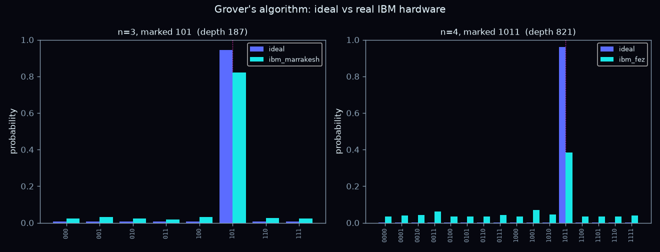
Both circuits have nearly the same ideal success (~0.95), so the only thing separating an 82% win from a 38% one is circuit depth: each Grover iteration carries a multi-controlled phase gate that compiles into a long chain of two-qubit gates, and the 4-qubit search runs 4.4× deeper (821 vs 187 gate layers). More depth means more time for the fragile quantum state to decohere.
There's a tell that it's still real Grover and not random noise: in the noisy 4-qubit run, the lost probability piles up in 1001 and 0011 — the strings exactly one bit-flip away from the target 1011. That's the fingerprint of single-qubit errors late in the circuit, the same "watch the limitation, don't hide it" honesty as the noise in the experiments above.
Quantum-generated art · a true hardware QRNG
One more hardware run, for fun. Eight qubits are put into an equal superposition with Hadamard gates and measured — each shot collapses to a uniformly random byte. This is a genuine quantum random-number generator: the bits come from physical measurement, not a software pseudo-random algorithm. I pulled 600,000 random bytes off ibm_marrakesh (a 156-qubit QPU) in one job and used them to drive these images.
You can even see the hardware in the statistics. A simulator's bytes sit almost perfectly at the ideal balance; the real device leans slightly toward 1s because physical qubits have readout error:
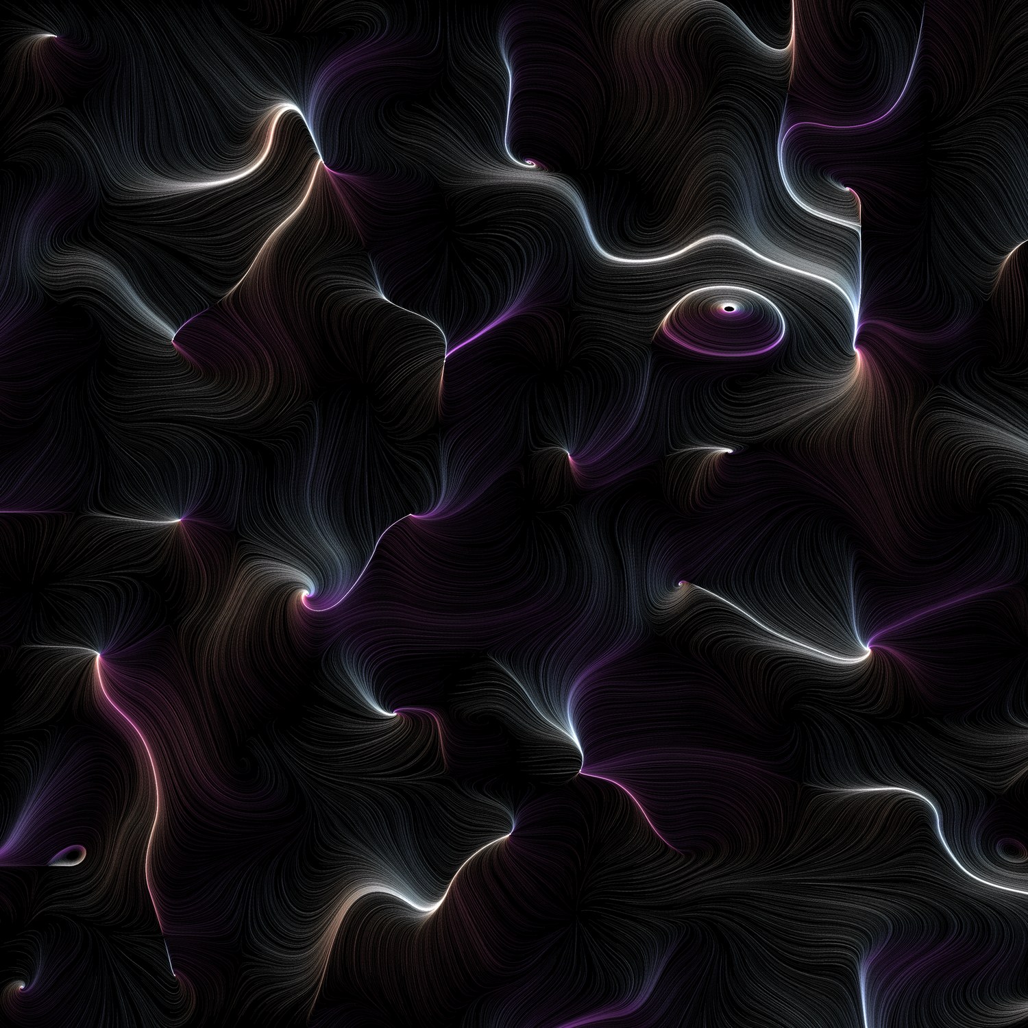
Quantum flow field
A coarse grid of angles is read straight from the quantum bytes, then smoothly interpolated into a vector field. Thousands of particles — seeded at quantum-random positions — flow along it, coloured by direction. Every angle and seed is a qubit measurement.
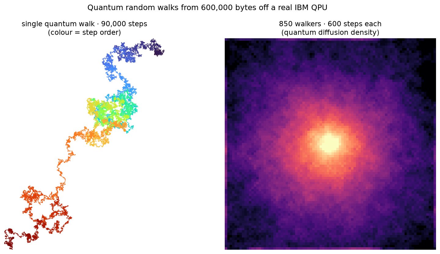
Quantum random walks
The same bytes as walk steps: one long walker tracing a Brownian thread (left, coloured by step order), and 850 walkers diffusing from the centre into the 2-D diffusion kernel (right).
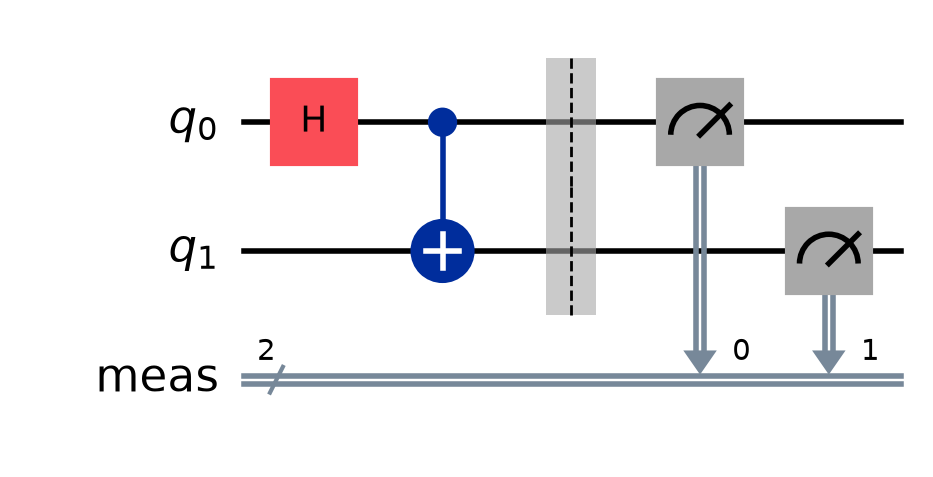
The circuit behind it
The whole QRNG is just this: Hadamard every qubit, then measure. Eight qubits give one random byte per shot.
How it works
- Feature map → kernel: each data point
xis encoded by a parameterized circuit into a quantum state|φ(x)⟩. The kernelK(x,y) = |⟨φ(x)|φ(y)⟩|²is the fidelity between two such states — computed exactly by statevector in the browser, and on hardware via a "compute-uncompute" circuit whose probability of measuring all-zeros equals that fidelity. - Hybrid model: the quantum kernel feeds an ordinary classical SVM (scikit-learn). The quantum computer only does the part it might one day be good at — embedding data into an exponentially large space.
- Real hardware, honest results: jobs run on IBM's free Open Plan against
ibm_fez. There's no quantum advantage here — on these small problems a classical model matches or beats it — but it's a faithful, hands-on tour of how the field actually works today. - Browser simulator: the live demos are a from-scratch complex statevector simulator (H, X, phase and CNOT gates) — no libraries, a few dozen lines of JavaScript.